ACT IntegratedExample

From GersteinInfo

ACT Integrated Example: Whole-Genome ChIP-Seq experiments

Here we describe how to use ACT on a set of two large example files from ChIP-Seq experiments.

To begin, download the signal files (from Gerstein Lab's PeakSeq project) here:

http://archive.gersteinlab.org/proj/PeakSeq/Scoring_ChIPSeq/Results/PolII/Signal_Maps/PolII/

http://archive.gersteinlab.org/proj/PeakSeq/Scoring_ChIPSeq/Results/STAT1/Signal_Maps/STAT1/

These are zipped signal files for PolII and Stat1. After unzipping the files for each transcription factor, it is useful to cat the signal tracks for the individual chromosomes together so that all the signals are in only two files. In this walkthrough they will be referred to as PolII.sgr and Stat1.sgr.

• Aggregation

After downloading the agg-py package, it is necessary to download an annotations file with coordinates you want to aggregate over. For this example, we used all transcription start sites as taken from build 18 of the human genome annotated by the gencode project.

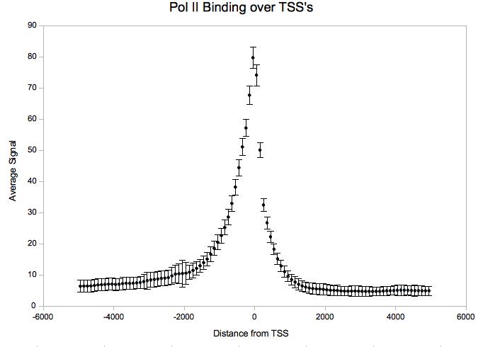
Using ACT.py, we get a four-column file which can be plotted in Excel or using R:

• Correlation

For this example, since we are dealing with signal tracks rather than SNP positions or a bed file of genomic locations, we will use the correlation tool found in corr-sat-bundle to do the correlation calculation. First, it is necessary to convert the signal tracks from sgr to wig format. A script which does this can be found here:

http://act.gersteinlab.org/sgr2wig.pl

Once we have converted both the PolII and Stat1 sgr files to wig files, we can change the parameters in correlation.sh so that the input files are "PolII.wig" and "Stat1.wig"

In addition, it is important to change config.txt so that the list of genomic regions includes all chromosomes, including mitochondrial sequences. (When the package is first downloaded, all lines except for the one denoting chromosome 22 are commented out).

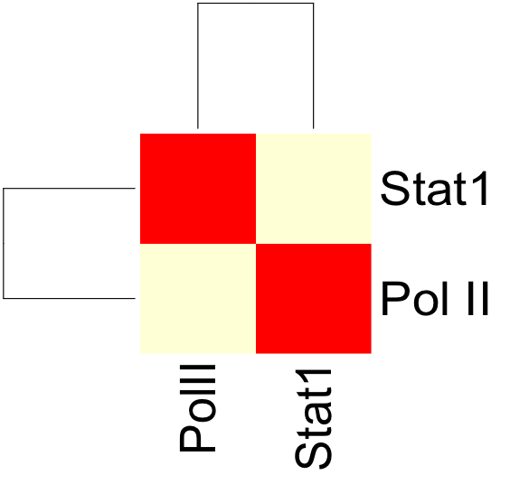
Once both the correlation.sh and config.txt files have been modified, we can run correlation.sh. This will produce an output file with a correlation matrix describing the correlation coefficients between PolII and Stat1 signal.

The resulting correlation matrix can be plotted in R using the heatmap function:

• Saturation

It is necessary to convert the wig files to bed files without a "signal" component. The following script takes wig files and converts them into bed files, with coordinates representing the regions of the signal track which are above a certain threshold (in this case 20).

http://act.gersteinlab.org/wig2bed.pl

Go to saturation.sh and change the input files to PolII.bed and Stat1.bed. It will also probably be necessary to change the alloted memory (in the second of the final java command in saturation.sh, change the numbers in the second field from 128 to 4096). Since there are only two signal tracks, the Saturation and Correlation analyses provide overlapping information.